Accompanying repository to the manuscript titled "Let us walk on the 3-isogeny graph: efficient, fast, and simple".
Table of contents
- Introduction
- Setup Process
- Benchmarking
- Reproducing the Manuscript Results
- Source-Code Technical Documentation: Doxygen
- Integrated CI/CD: Build, Test, Benchmarking, and Reporting
- How to use our Docker container?
- Additional Resources' Build Process
- Conclusions, Acknowledgements and Authors
1. Introduction
Our paper reached several important results:
- This work centers on improving HASH functions (CGL Function), KEMs (QFESTA) and NIKEs (CTIDH).
- Our results help to propose friendly parameters for QFESTA, along with the first efficient implementation in C of the radical 3-isogenies.
- Our results speedup the dCTIDH-2048 by a 4x factor, without any considerable change in the parameter sets and allowing a straightforward integration (just replacing small isogenies of degree 3,5,7,11 and 13 by the aforementioned radical 3-isogenies).
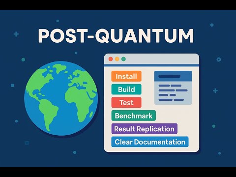
A video summarizing our ideas and contribution (in a general-reader level) is shown below:

The YouTube link of our video is shown here: Let us walk on the 3-isogeny graph: efficient, fast, and simple
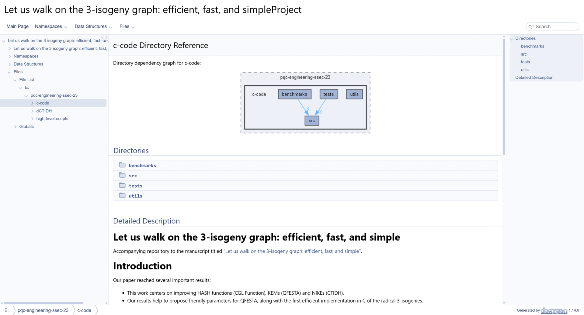
A general tree description of the source code of our project is shown below.
In the following sections, we will cover in detail:
- How to build, test, and benchmark,
- How to replicate the results reported in the manuscript,
- How to generate the source code technical documentation using Doxygen,
- A real-life production CI/CD pipeline integration, showing how to download our manuscript's results as public artifacts, and
- Detailed instructions on how to download and mount our Docker container.
A detailed (full) video tour of our artifact is shown here: Let us walk on the 3-isogeny graph: A (full) guided tour of our GitHub Artifact
For convenience, a list of all the videos of each individual section is shown below.


A slide-style presentation with a summary of the technical steps presented in this repository is also available here: Let us walk on the 3-isogeny graph: Step-by-step Artifact Walkthrough.
2. Setup Process
In this section we present a setup process that can be run in any Linux terminal. In case a specialized IDE like CLion is desired, please refer to Let us walk on the 3-isogeny graph: CLion Setup.
2.1. System requirements
Our (physical) testbed consists of machine with a 12th Gen. Intel(R) Core(TM) i9-12900H CPU and 32 Gb of RAM, running Ubuntu 20.04.6 LTS (64 bits), but any Linux environment running in an Intel CPU is enough. Currently, only Intel CPUs are natively supported. To run our project in Apple Silicon-based computers, please refer to Section 7: How to use our Docker container?.
Our project works in any out-of-the-box Linux-based environment with some basic software requirements:
- Cmake
- Python3 (numpy and matplotlib)
To install all our required software dependencies, execute
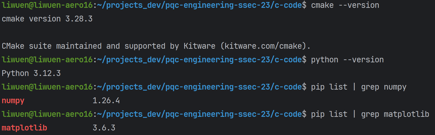
To check if your system counts with the required software, simply run
If all the requirements are met, the terminal should return installed versions like the ones below.
2.2. Build
To build our project, in the root directory pqc-engineering-ssec-23, simply run
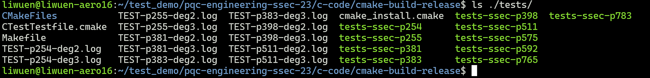
This will create the cmake-build-release folder with all the tests for all the supported primes: p254, p255, p381, p383, p398, p511, p575, p592, p765, and p783. A list of the generated tests is shown below.
A demo of the whole process of setup and build process is shown below.
2.3. Testing
In this section, we show how to perform the testing of our source code. For a detailed explanation of each testing mode, please refer to our additional documentation: Let us walk on the 3-isogeny graph: (Detailed) Build, Test and Benchmarking Framework Documentation.
After building as shown in the previous section, inside the c-code/cmake-build-release folder, locate all the possible tests with
To execute any particular test, simply select one of the following
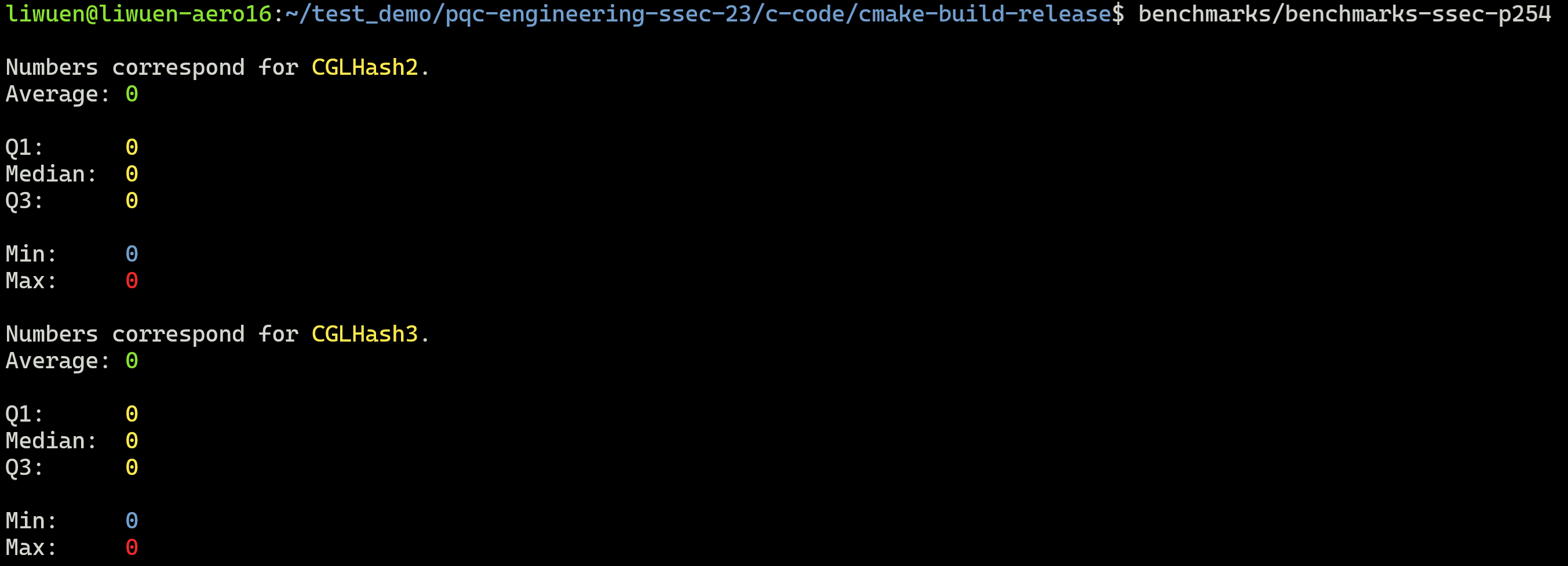
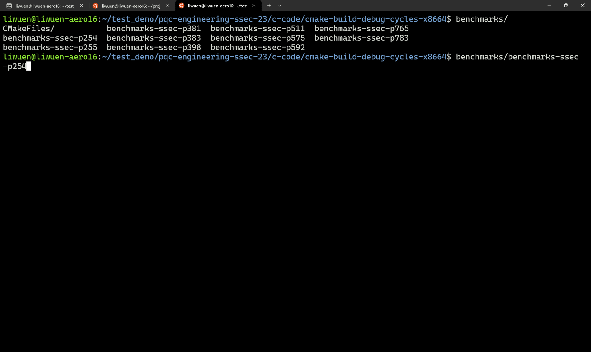
For example, the execution of ./tests/tests-ssec-p254 is shown below.
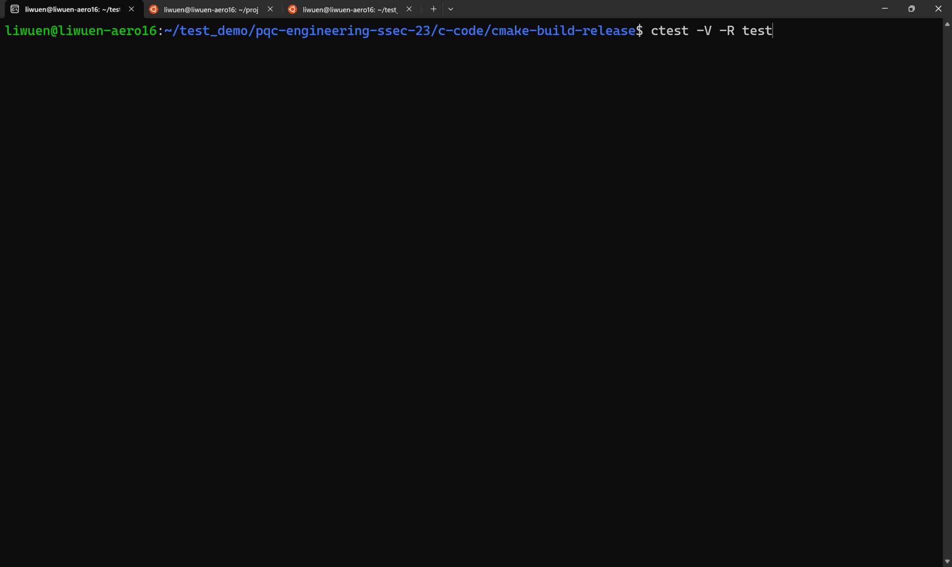
To run ALL the tests in verbose mode, simply run
A demo of all the tests running in verbose mode is shown below.
3. Benchmarking
In this section, we show how to perform the benchmarking of our source code.
As supplementary material:
- A detailed walkthrough of the steps in this section is available in our YouTube video: Modulo 3: How to benchmark our project? The Dos and Dont's.
- For an explanation of how to perform the benchmarks in a detailed mode (and more insights about the used CPU benchmarking method), please refer to our additional documentation: Let us walk on the 3-isogeny graph: (Detailed) Build, Test and Benchmarking Framework Documentation.
For benchmarking, the correct commands must be used when doing the first cmake. Inside the root directory pqc-engineering-ssec-23, simply run
followed by
NOTE: Benchmarking does not work for
In case you run the benchmarking in either one of these two build modes (without the -DBENCHMARKING and the -DARCHITECTURE flags), you will get the following error:
To execute any particular benchmarking, inside the cmake-build-release-cycles-x8664 folder, simply select one of the following
A demo of successful benchmarkings is shown below.
4. Reproducing the Manuscript Results
In our manuscript, several statistical figures are shown. In this section, we cover how to replicate the obtained graphs.
As supplementary material, a detailed walkthrough of the steps in this section is available in our YouTube video: Modulo 4: How to Replicate our Manuscript's Results?
In order to reproduce some of the figures in the manuscript, we provide with easy-to-use scripts that wrap all the required executions of the benchmarking tests, and by using numpy and matplotlib, generate the manuscript graphs.
The related code to reproduce our results is shown in the tree below.
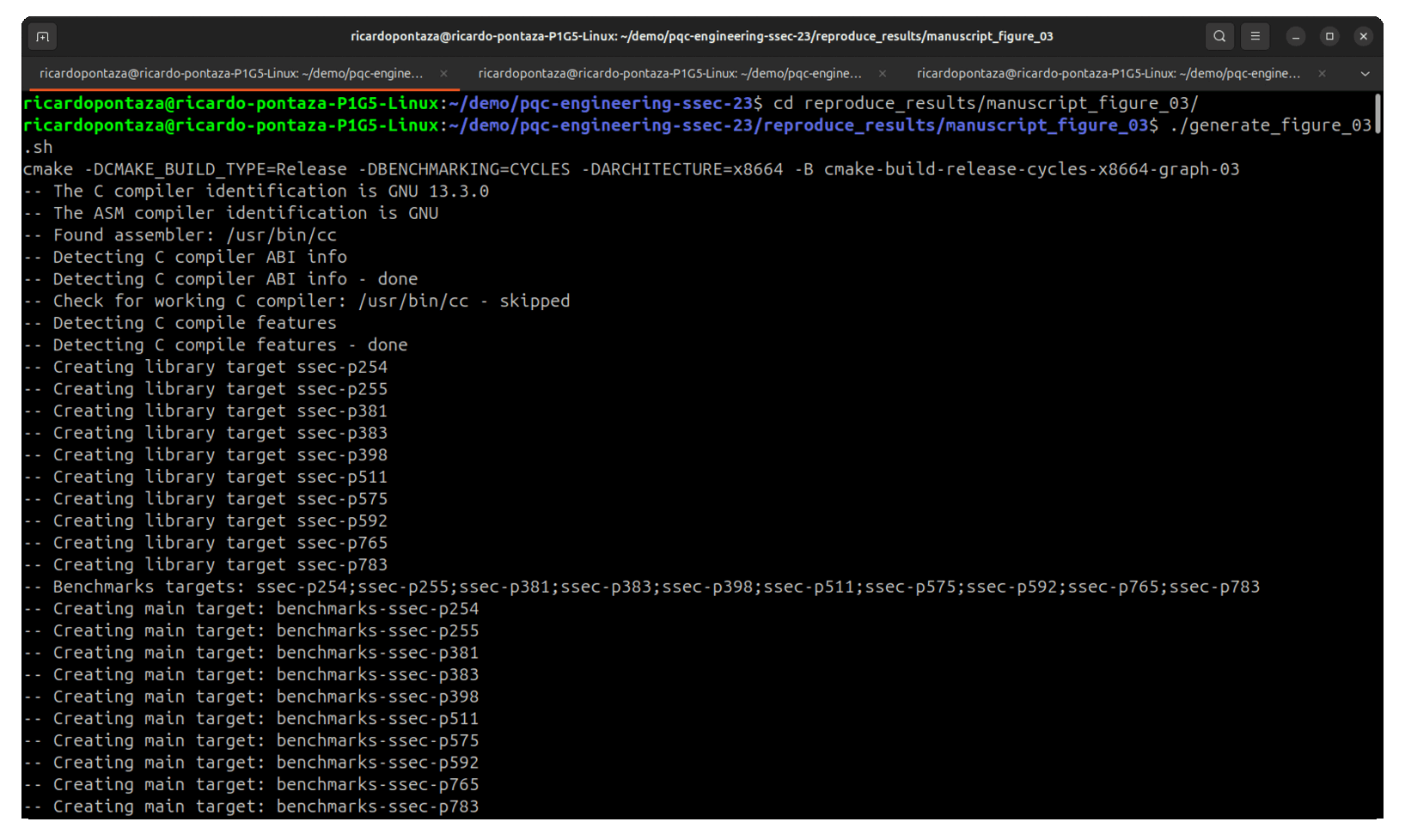
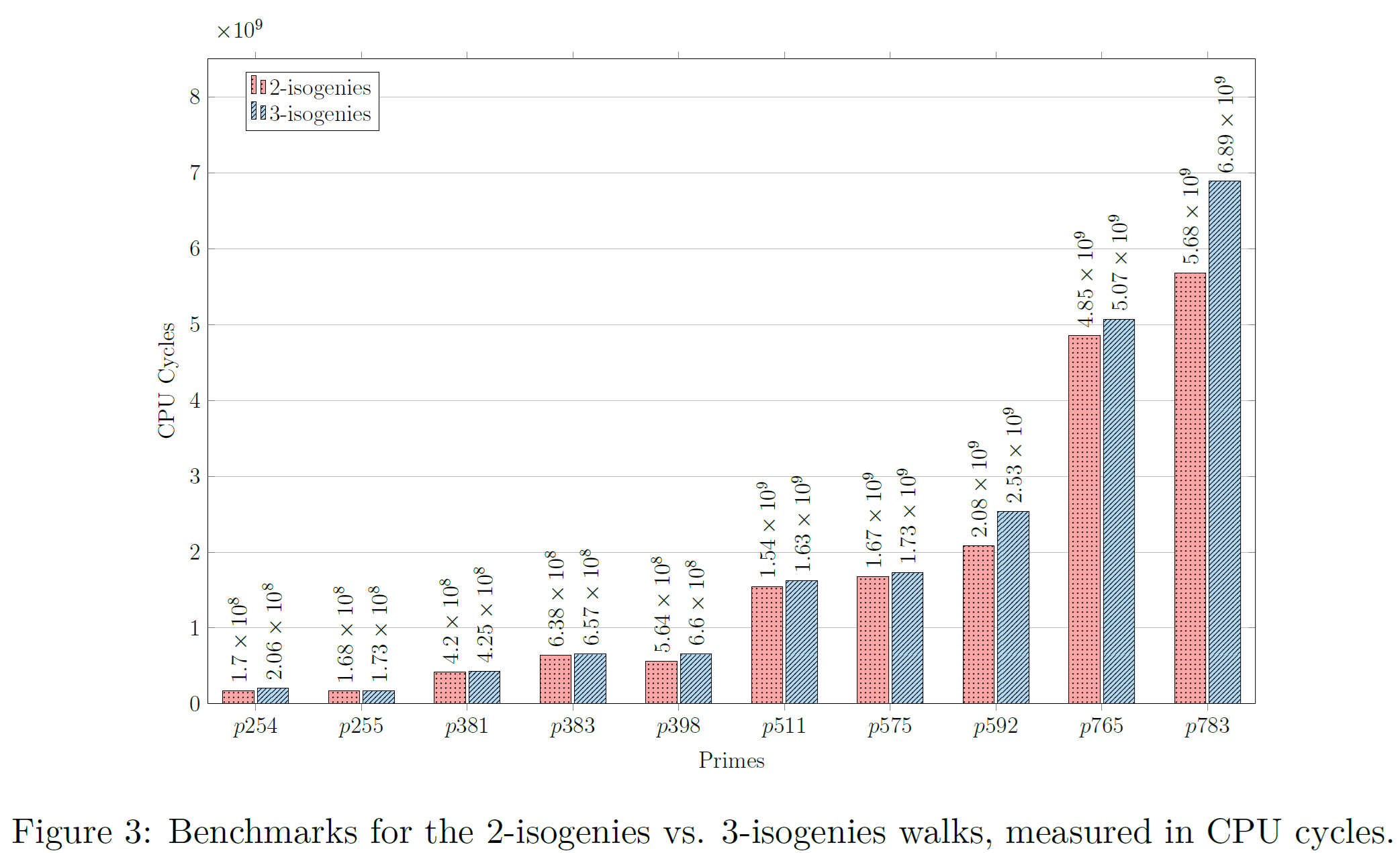
4.1. Figure 3: Benchmarks for the 2-isogenies vs. 3-isogenies walks
Inside the reproduce_results/manuscript_figure_03 folder, it is necessary to give execution permissions to the script, via
Then, just simply execute it
This will automatically build with the -DBENCHMARKING=CYCLES -DARCHITECTURE=x8664 flags, and perform all the statistics. At the end, a bar graph is automatically generated.
A demo of how to obtain the manuscript's Figure 03 is shown below.
where the original Figure 3 presented in the manuscript is shown below.
A PDF is generated with the generated graph and stored inside the reproduced_results/generated_figures/figure_03_output folder. This folder will be automatically generated once the generate_figure_03.sh script executes successfully.
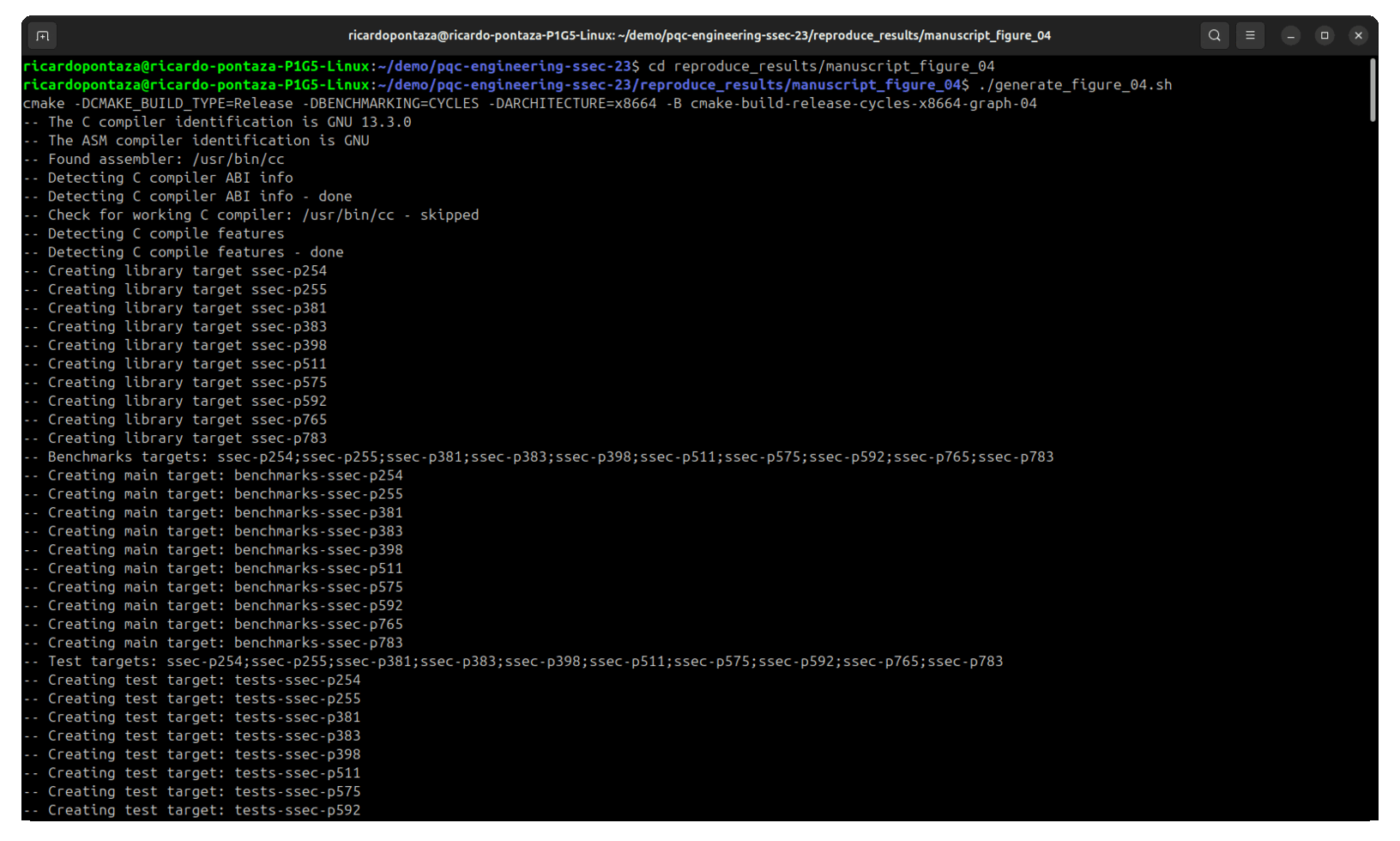
4.2. Figure 4: Benchmarks for the 3-isogenies walks (Our solution vs. QFESTA)
Similar to the previous figure, inside the reproduce_results/manuscript_figure_04 folder, it is necessary to give execution permissions to the script, via
Then, just simply execute it
This will automatically build with the -DBENCHMARKING=CYCLES -DARCHITECTURE=x8664 flags, and perform all the statistics. At the end, a bar graph is automatically generated.
A demo of how to obtain the manuscript's Figure 03 is shown below.
where the original Figure 4 presented in the manuscript is shown below.
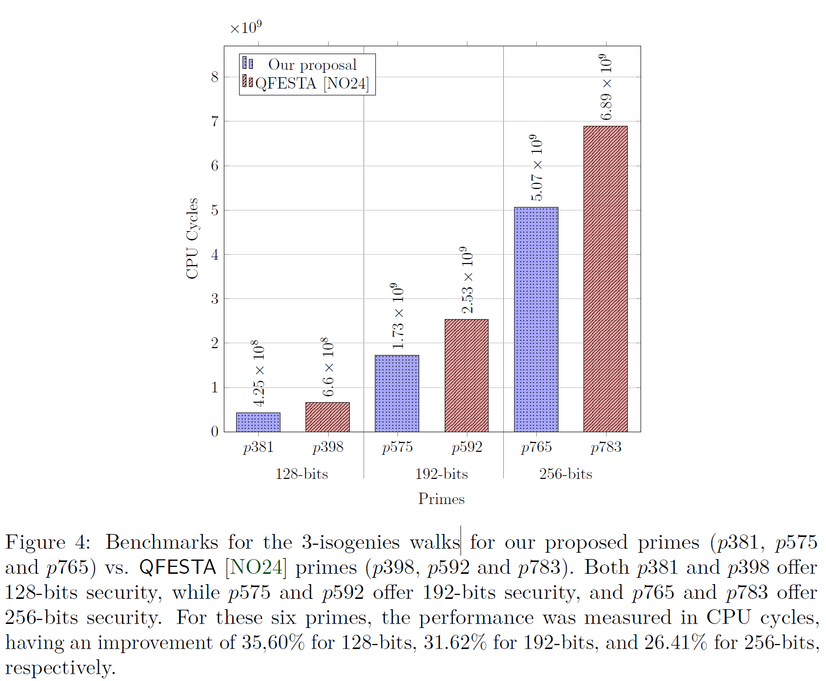
A PDF is generated with the generated graph and stored inside the reproduced_results/generated_figures/figure_04_output folder. This folder will be automatically generated once the generate_figure_04.sh script executes successfully.
4.2. Figure 5 (a) and Figure 5 (b): Benchmarks for state-of-the-art dCTIDH vs. dCTIDH modified using our proposal.
Similar to the previous figures, inside the reproduce_results/manuscript_figure_05 folder, it is necessary to give execution permissions to the script, via
Then, just simply execute it
This will automatically create three folders:
The script will generate all the required folders to perform all the statistics. At the end, two line graphs are automatically generated. The first graph is the one associated to Figure 5 (a) in the manuscript, while the second graph is Figure 5 (b).
A demo of how to obtain the manuscript's Figure 05 is shown below.
where the original Figure 5 presented in the manuscript is shown below.
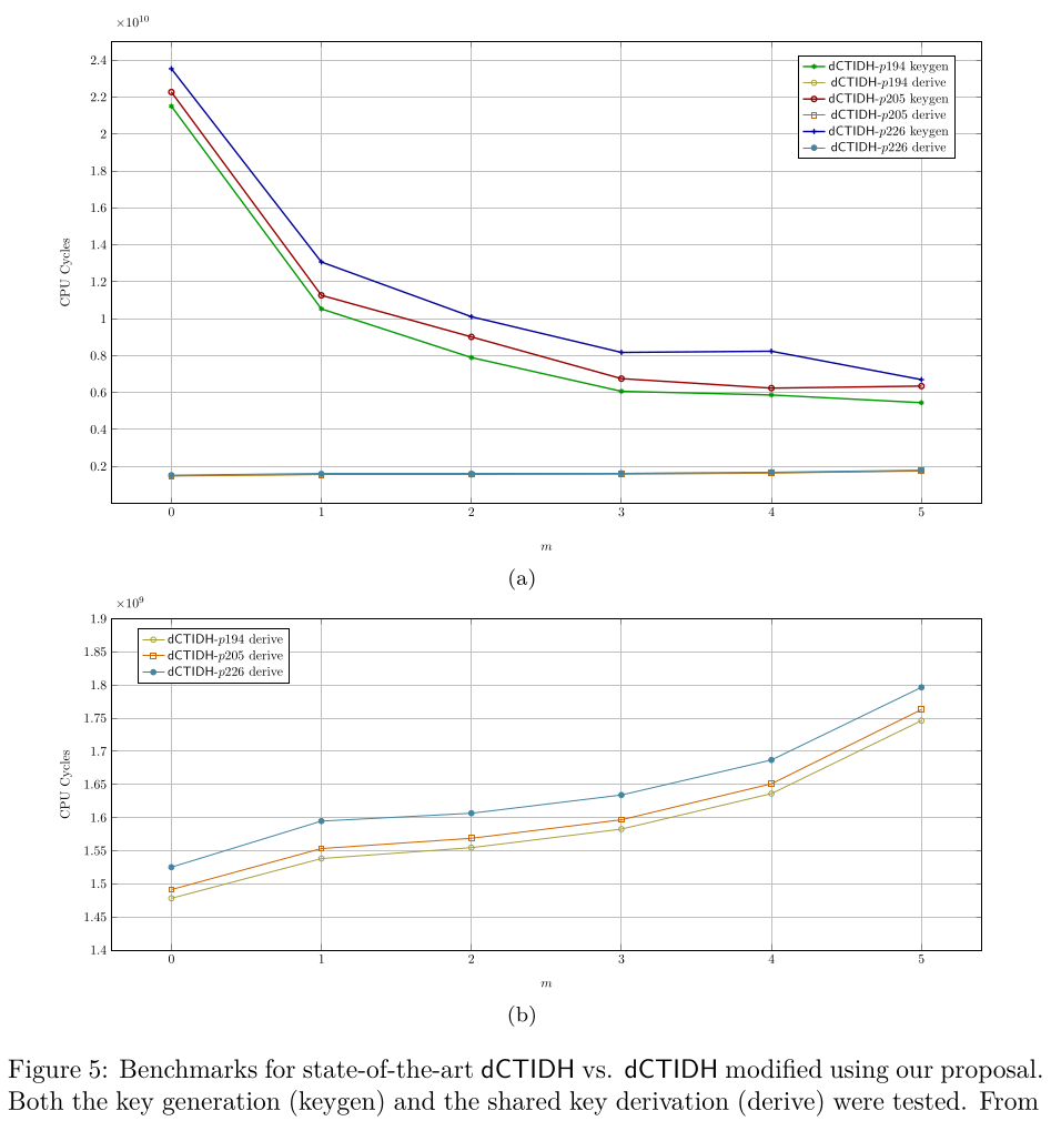
Two PDF files are generated with the generated graphs and stored inside the reproduced_results/generated_figures/figure_05_output folder. This folder will be automatically generated once the generate_figure_05.sh script executes successfully.
5. Source-Code Technical Documentation: Doxygen
Our project supports automatic technical documentation generation via Doxygen. As supplementary material, a detailed walkthrough of the steps in this section is available in our YouTube video: Modulo 5: How to Generate the Source Code Technical Documentation?
To install Doxygen (and Graphviz) in case not installed in the system, simply run
To generate the Doxygen documentation, inside the docs folder, simply run
This will generate an HTML site with interactive diagrams, and plenty of technical documentation. A demo of the generated documentation is shown below.
A link to a public-hosted version of our source-code documentation is shown here: Let us walk on the 3-isogeny graph: Technical Documentation.
6. Integrated CI/CD: Build, Test, Benchmarking, and Reporting
To prove that this project can be integrated in an industrial environment where Continuous Integration (CI) and Continuous Delivery (CD), we follow a classic CI/CD workflow of (1) Build, (2) Test, (3) Benchmark, and (4) Reporting.

As supplementary material, a detailed walkthrough of the information conveyed in this section is available in our YouTube video: Modulo 6: CI Pipeline in action: Real-World Software Development Demo.
To provide CI/CD related capabilities, in our source code we provide a cmake-multi-platform.yml file that uses Docker images to build, test and benchmark our solution. This is done to prove that our code and contribution can be integrated in a pipeline and be delivered as a part of a cryptographic solution in an industrial scenario.
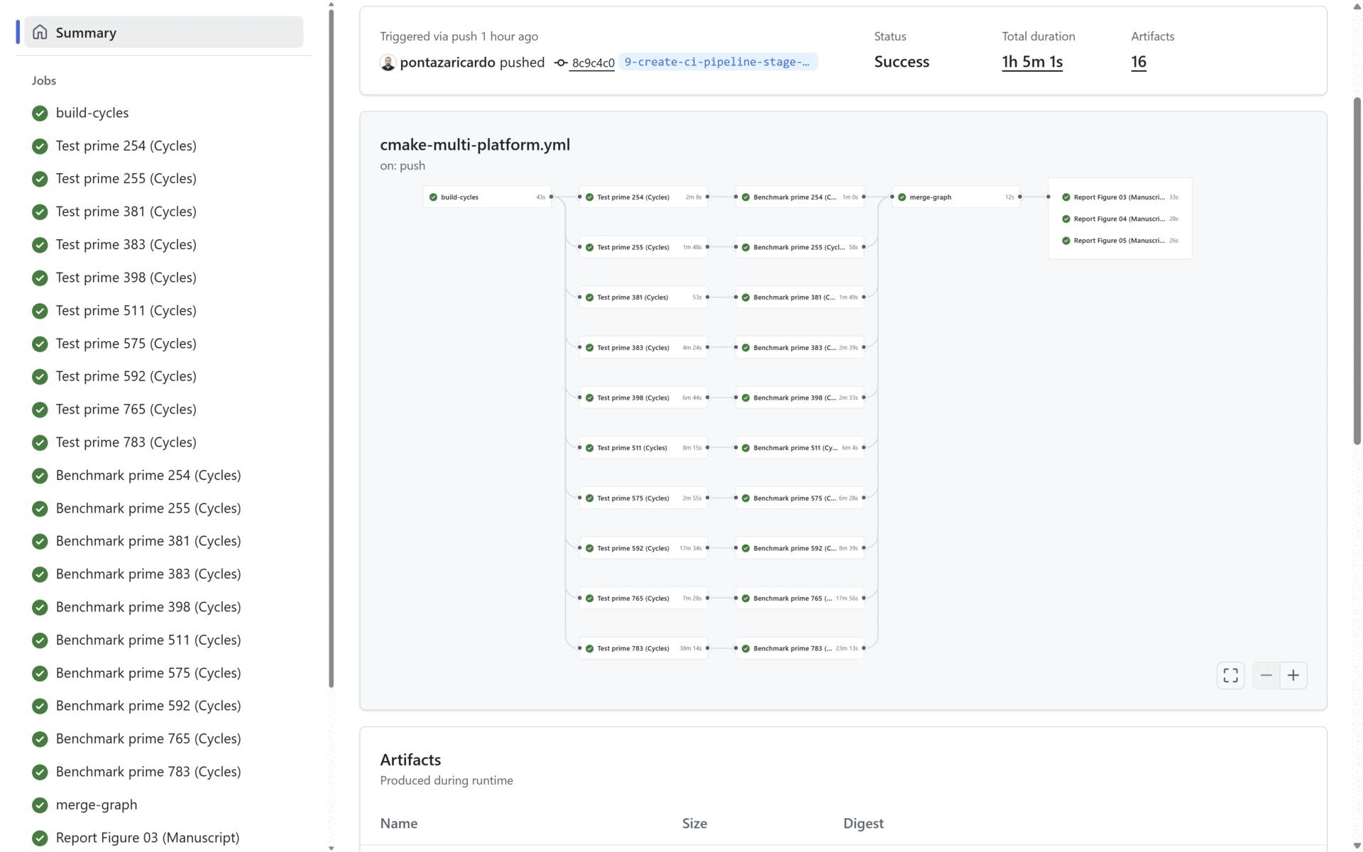
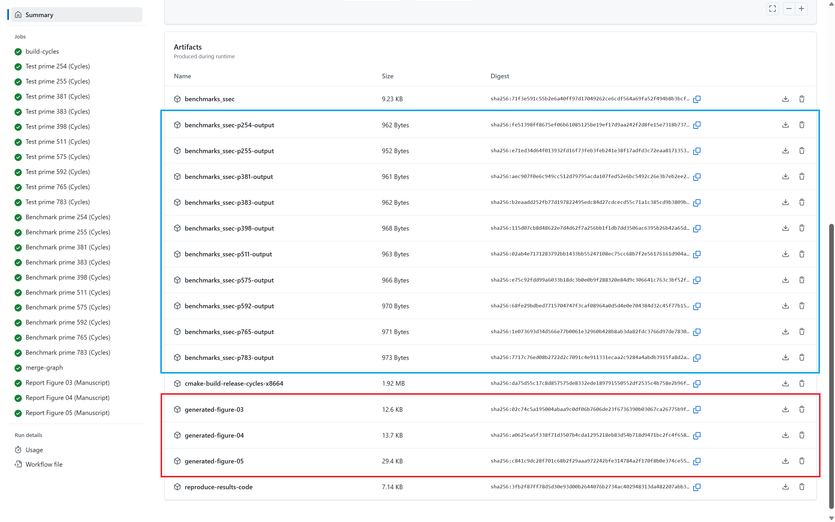
At the end of the Benchmark stage, the Reporting stage generates the three graphs presented in the manuscript (See Section 4: Reproducing the Manuscript Results). All three generated graphs and all the benchmarking results (per prime) are uploaded as artifacts in the pipeline. In the figure below:
- The benchmark statistics are uploaded in the artifacts marked in blue, and
- The generated manuscript graphs are uploaded in the artifacts marked in red. All the statistical data and all the graphs are uploaded as public artifacts to provide means to the reader to replicate our results.
For our project, the list of executed CI pipelines is shown here: GitHub Pipeline, and an example of a successful pipeline execution with the publicly uploaded artifacts (Statistical results and generated graphs) is shown here: Pipeline Execution Example.
7. How to use our Docker container?
For the convenience of our readers and any scientist that would like to replicate our results, we provide (1) a publicly available Docker container, and (2) the Docker file used to build it. These two offer our readers the options to download and/or locally build the Docker container with all our software requirements. This provides a self-contained environment where our artifact runs out-of-the-box.
As supplementary material, a detailed walkthrough of the steps in this section is available in our YouTube video: Modulo 7: How to Download our publicly available Docker Container?
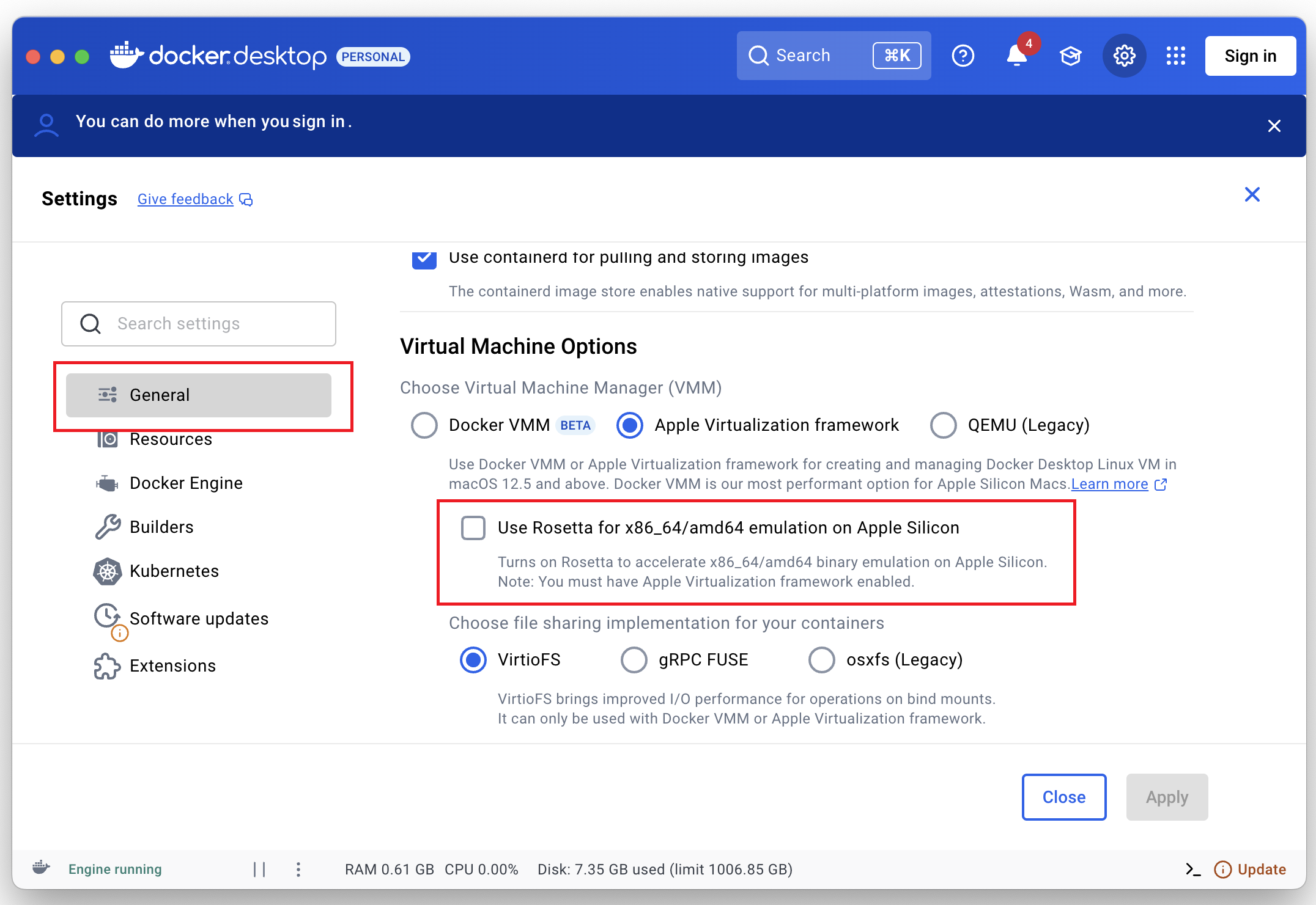
Currently, natively only Intel CPUs are supported. To build, test, benchmark and replicate our results in Apple Silicon-based computers (M1, M2, M3, M4 CPus), in Docker Desktop, turn OFF Rosetta as shown below.
7.1. How to download our public Docker container?
To download our Docker container, simply execute the command below
and to verify that it was downloaded correctly, execute
7.2. How to locally build our Docker container?
In case it is desired to locally-build the container, the required Dockerfile can be found here (location: docs/Dockerfile).
To build the local Docker container, simply execute
and to verify that it was built correctly, execute
7.3. How to mount our Docker container?
To mount the Docker container, first locate your terminal at the artifact's root folder(pqc-engineering-ssec-23), and then:
- In case the Docker container was downloaded, execute docker run --rm -ti -v $PWD:/src -w /src tiicrc/github-selfhosted-runner-pqc:latest bash
- In case the local container was built, then execute After mounting, for either of both cases mentioned above, the terminal will change todocker run --rm -ti -v $PWD:/src -w /src pqc-engineering-ssec-23-local-docker:latest bash/src# <insert commands here>
At this point, all the steps presented in Section 2: Setup Process, all the benchmarking shown in Section 3: Benchmarking, all the experiments presented in Section 4: Reproducing the Manuscript Results, and all the steps to generate the technical documentation using Doxygen as shown in Section 5: Source-Code Technical Documentation: Doxygen shall work without problems.
For Apple Silicon-based computers, in case the error illegal instruction is returned, please modify the Rosetta settings described above.
8. Additional Resources' Build Process
As mentioned before, for a detailed explanation of our testing and benchmarking frameworks (with insights of the CPU benchmarking approach), please refer to our additional documentation: Let us walk on the 3-isogeny graph: (Detailed) Build, Test and Benchmarking Framework Documentation.
As part of our experiments, we used a modified version of dCTIDH. To build the modified dCTIDH, please refer to Let us walk on the 3-isogeny graph: dCTIDH modified version.
9. Conclusions, Acknowledgements and Authors
We sincerely thank the scientific community, our collaborators, and everyone who made our artifact possible — with special gratitude to our DevOps team for their invaluable work in setting up our self-hosted runner and infrastructure. Words alone cannot fully convey our gratitude to our collaborators. To express our conclusions and acknowledgments in a more vivid and engaging way, we invite to watch our video here: Modulo 8: Conclusions.
This project highlights the importance of clear, comprehensive documentation, building software that seamlessly integrates into continuous integration pipelines to meet industry standards, and leveraging Docker containers for reproducibility.
We invite fellow researchers and practitioners to explore, test, and expand upon our work, helping it grow and evolve in new directions. For further information, please feel free to contact any of the authors: